
The y-axis is 90 degrees in an anti-clockwise direction from the x-axis.
It may not be enough to describe an objects position by just x and y coordinates, it is desirable to also have orientation. Can do this by attaching a coordinate frame to the object. Now the objects orientation is described by the orientation of the attached coordinate frame with respect to the reference (world) coordinate frame.
Can describe the motion of an object in two steps:
It is convention that the x-axis is in the direction of normal motion for the machine.
May be represented with this symbol, pronounced ksi,
\[\xi\]
where \(\xi\) is
\[(x,y,\theta)\]
\(^{A}p_B\) where p is the vector to point B with respect to (from) A.
\(^{A}\xi_B\) where \(\xi\) is the pose of B with respect to A.
Use pose to describe a coordinate frame with respect to another coordinate frame. Use a vector to describe a point with respect to a coordinate frame.
We can’t add poses and vectors.
If you have a pose \(^{W}\xi_C\) and a vector \(^{C}p_d\), then to find \(^{W}p_d\) you must transform the vector from one frame to another like
\[^Wp_d = ^W\xi_C \cdot ^Cp_d\]
Relative poses can be compounded or composed i.e. they can be ‘added’.
We use the symbol \(\oplus\) for this, e.g.
\[^A\xi_C = ^A\xi_B \oplus ^B\xi_C\]
You can use a pose graph to better display and easily compute the relationships between the all of the poses. A pose graph is a directed graph, with solid edges between coordinate frames (nodes) indicating that the pose is known, and a dotted line indicating that the pose is unknown but perhaps it may be computed.
You can define an unknown pose with a composition of the known poses.
If when finding a pose it is necessary to travel backwards (in the reverse direction) in the graph, that may be represented using the symbol \(\ominus\).
\[^X\xi_Y \oplus ^Y\xi_Z = ^X\xi_Z\]
\[^Xp = ^X\xi_Y \cdot ^Yp\]
\[\xi_1 \oplus \xi_2 \neq \xi_2 \oplus \xi_1\]
\[\ominus ^X\xi_Y = ^Y\xi_X\]
\[\begin{aligned} \xi \ominus \xi &= 0 & \ominus \xi \oplus \xi &= 0 \\ \xi \ominus 0 &= \xi & \xi \oplus 0 &= \xi \end{aligned}\]
Here \(^Ap\) and \(^Bp\) share an origin and so are the same. Equating these two gives

which can be written in matrix form like

which can be more concisely written as
\[^A\boldsymbol{p} = \mathbf{R} ^B\boldsymbol{p} \qquad\text{ where } \mathbf{R} = \begin{pmatrix} \cos{\theta} & -\sin{\theta} \\ \sin{\theta} & \cos{\theta} \end{pmatrix}\]
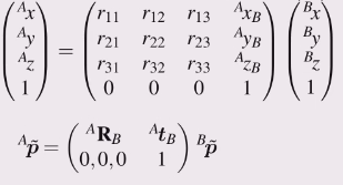
but write it using the notation
\[^A\boldsymbol{p} =\ ^A\mathbf{R}_B \ ^B\boldsymbol{p} \qquad\text{ where } ^A\mathbf{R}_B = \begin{pmatrix} \cos{\theta} & -\sin{\theta} \\ \sin{\theta} & \cos{\theta} \end{pmatrix}\]
So R is a rotation matrix that
To rotate a vector from frame {A} to frame {B} we use the inverse rotation matrix, which for a rotation matrix is simply the transpose.
Also note the equivalence
\[^B\boldsymbol{R}_A =\ ^A\boldsymbol{R}^{-1}_B\]

t is for translation.
I think a 3x3 matrix is preferred in the last step because then you can take the inverse (the zeros and ones in that last row are constant).


Remember the order when transforming:

Pose is a matrix \(^A\xi_B \sim\ ^A\boldsymbol{T}_B\)
Compounding (composition) (\(\oplus\)) is a matrix-matrix product.
Negation (\(\ominus\)) is a matrix inverse.
Vector transformation (\(\cdot\)) is a matrix-vector product.
\[\xi\cdot p \rightarrow \boldsymbol{T} \widetilde{p}\]
The pose notation using \(\xi\) is exactly the same as in 2D, and the same rules apply.
The difference is in the implementation.
Frames {A} and {B} share the same origin.
![]()
For rotation about either the x, y or z axis.
Multiplying these in various combinations will achieve much more complicated rotations.
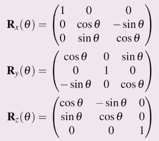
The order in each rotations are applied in 3D is critically important; they are non commutative.
(Paraphrased)
Any rotation can be expressed by a sequence of rotations (not more than three), where no two successive rotations are about the same axis.
These are the set of rotations where there are two rotations about the same axis (but not sequentially).
XYX, XZX, YXY, YZY, ZXZ, ZYZ
ZYZ is commonly referred to as ‘Euler angles’, but mind it is only one of the six possible.
Euler angles are not unique a representation of orientation in space.
Rotate on new axis.
For the Euler angle approach, the order of the matrix multiplication and transformations are the same as the order they occur.
These are the remaining sets of rotation sequences which satisfy Euler’s rotation theorem. All rotations are about different axes.
They are
XYZ, XZY, YXZ, YZX, ZXY, ZYX
XYZ and ZYX are both commonly referred to as roll pitch yaw angles. Which one is referred to depends on the context. XYZ seems to be the default for Robotics M course.
Rotate on original axis.
For fixed angle approach: the order of transformations (including translation) should be all reversed. Say a frame {B} is located as follows: initially coincident with a frame {A}, we perform a rotation about ZA axis, followed a rotation about YA axis, followed by a translation along [XA, YA, ZA].
Then the transformation matrix (4X4) is: Trans[XA, YA, ZA].Rot(YA).Rot(ZA)
Also known as Gimbal lock.
A Gimbal is a mechanism used to stabilise some device to space.
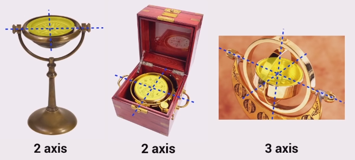
Gimbal lock is when two of the axis become aligned.
For roll-pitch-yaw angles, Gimbal lock occurs when pitch is at \(\pi/2\). Results in rotation axes of the first and third rotations (roll and yaw) parallel.
For example, the set of roll-pitch-yaw angles (30, 90, -20)° is equivalent to the set (0, 90, 10)°. A pitch of 90° results in Gimbal lock, whereby the roll and yaw axes become aligned, and thus rotations about these axes can be summed and by convention assigned to the yaw angle.
To minimise Gimbal lock, choose coordinate conventions so that the pitch angle is around 0 for normal operating conditions.
Describes the orientation of the end effector.
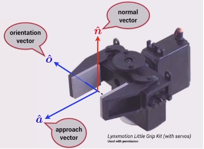
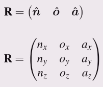
All three columns of the rotation matrix are orthogonal, hence one of the vectors can be computed from the other two.
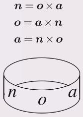
The orientation of a body in 3D can also be described by a single rotation about a particular axis in space.
Need to know the axis of rotation vector \(\boldsymbol{v}\), and the angle of rotation about the vector \(\boldsymbol{\theta}\).
We observe that the axis around which the rotation occurs must be unchanged by the rotation, therefore the rotation axis must be an eigenvector of \(\boldsymbol{R}\).
A rotation matrix has three eigenvectors:
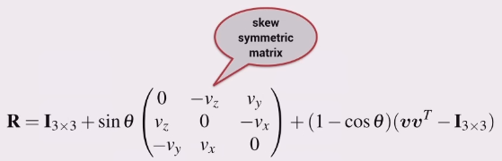
If you know \(\theta\) and the eigenvector, then the rotation matrix can be found using the Rodrigues equation.
Pose has
It can be represented by
Using the rotation matrix avoids singularity’s, unlike the Euler and fixed angle approaches.
A serial-link manipulator consists of a series of joints, each connected by a rigid link to the following joint.
A parallel-link manipulator consists of one or more joints on the base, each connected by a rigid link to the end-effector.
Other types: SCARA robot (Selective Compliance Articulating Robot), Gantry robot - overhead (x,y,z).
Robotic joints can either rotate or slide
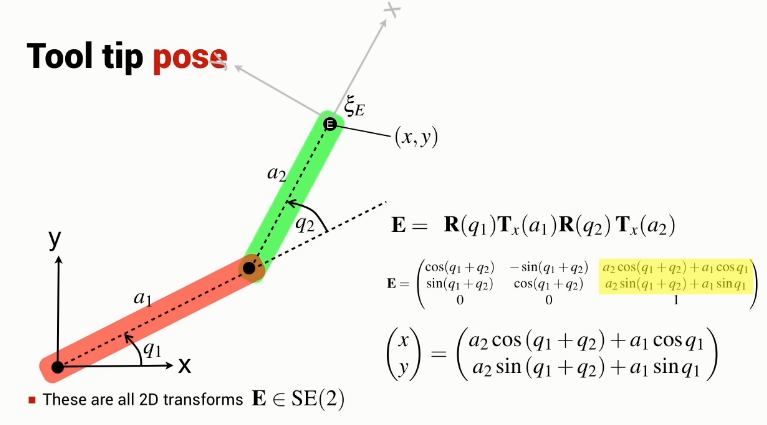
Get to the end effector frame by rotating and translating the reference coordinate frame.
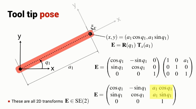
Both position and angle is a function of the angle \(q_1\) and so the position and angle cannot be set independently.
i.e. can move to any point lying on a circle
Same as for 1-joint, the orientation of the end effector is not independent from its position in the xy plane.
Always two joint angle configurations that result in the same end effector position.
Unlike the 1 and 2 joint planar robotic arm, the orientation and position of the end effector are independent.
There are an infinite number of joint configurations that result in an end-effector position.
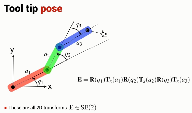
To find the end-effectors pose, the process is much the same as for a planar robot arm, multiply a bunch of rotation and translation matrices.
First identify the joints of the robot. Then a good way to figure out the order of the multiplications is to imagine the grippers/end-effector of the robot pointing up, coming out of the base of robot. Then imagine the rotations and translations as the end-effector approaches each joint.
q (joint configuration) is a vector of length N (number of joints) where the elements of q (joint coordinate) are either an angle or a length.
q belongs to the space C (space of all possible configurations), which is a subset of the N dimensional space.
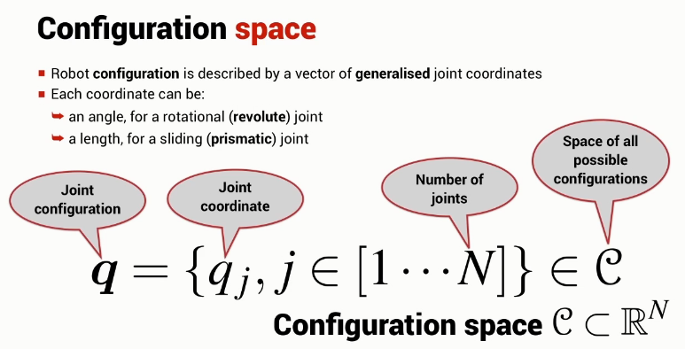
There is also the space of all possible end-effector poses, T.
The dimension of the configuration space is the robots degrees of freedom, i.e. the number of joints.
The dimension of the task space is the degrees of freedom in the task space.
In the three dimensional world (that we and our robots live), it is not possible to have a task space bigger than six.
To reach all of the task space dim C \(>=\) dim T
When dim C > dim T (especially when dim C >> dim T), the shape of the arm can be controlled as well as the position/orientation of the end-effector.
A general theory to describe an articulated sequence of joints.
Each joint in the robot is described by four parameters.
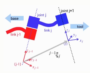
Denavit-Hartenberg notation describes the relationship between 3D coordinate frames attached to two successive links with four parameters.
For a robot with N joints the links are numbered from 0 to N, where link 0 is the fixed base of the robot.
A coordinate frame is attached to the far (distal) end of every link (closest to the end-effector)
The pose of a link frame is described with respect to the previous link frame
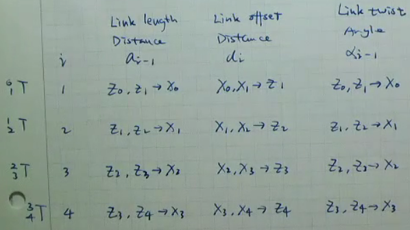
Four parameters: \(\theta, d, a, \alpha\)

There are constraints when using Denavit-Hartenberg notation:
Axis \(x_j\) intersects axis \(z_(j-1)\)
Axis \(x_j\) is perpendicular to axis \(z_(j-1)\)
6 parameters - 2 constraints = 4 parameters
Note that because of these constraints, a link coordinate frame may not necessarily lie on the physical robot.
The axis of each joint is defined by the z-axis of a coordinate frame
The joint rotates about the z-axis (revoltue joint), or
The joint translates along the z-axis (prismatic joint)
A table is used to represent each of the DH parameters for each joint.
A good way to remember how to find each of the parameters is to use the following table.
In reality, we want the end point of the robot to be the end of whatever tool is attached to the robot. Need to apply a tool transform to the end pose of the robot.
Also can apply a base transform to reposition or reorient the robot in space, i.e. flip the robot upside down etc.
The derived inverse kinematic function has two solutions
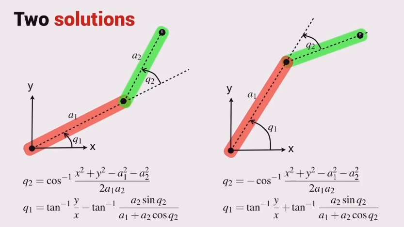
Determine the transformation matrix for the end-effector and pick out the translation parts. Now you have equations for x=… and y=… so then solve for the angles.
A 6-link industrial robot such as the Puma 560 has eight different arm configurations.
The arm can be in either a left-handed or right-handed configuration, 2 possible configurations. In addition the elbow can be either above or below the shoulder, another 2 possible configurations. Finally the gripper can be at a particular angle about the gripper axis, or the same angle plus 180 degrees — for a common two-fingered or parallel jaw gripper it makes no difference. This is another 2 possible configurations. In total there are 2x2x2 possible configurations, a total of 8.
A configuration change is a motion that starts and ends with the same end-effector configuration.
Used for switching from left-handed configuration to right-handed, and vice versa.
Many 6-DOF robots have a spherical wrist. This is where all 3 wrist joint axes intersect at a single point.
The analytic solution may be too hard to compute or not exist.
Initial conditions will determine the configuration of the end pose, trial and error may be needed, i.e. can’t guarantee a particular configuration.
Can be computationally expensive (iterative algorithm).
Numerical inverse kinematics works well for redundant robots.
Robot may not be able to reach the requested pose
Related to the Gimbal lock problem.
If particular axes are aligned, can loose a degree of freedom, affecting the robots ability to reach some positions.
Very high DOF robot.
Use a numerical approach to solve for joint angles.
How to smoothly move from one pose to another.
Simple approach.
No constraints on the path except for the start and end points
Determine the pose at each intermediate point
Results in straight line motion in 3D space.
Still, there is little difference between Cartesian interpolated motion and joint books interpolated motion.
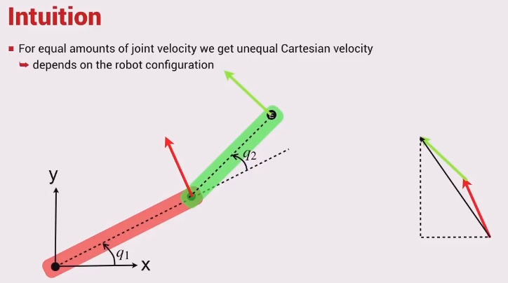
If the joints move at this particular joint velocity, what is the velocity of the end-effector?
Rate of change of a pose.
Find the expression for x and y (as a function of the joint angles) just like in when finding the inverse kinematics.
Make the joint angles functions of time
Take the derivative of x and y
Factor out the \(\dot{q_1}\) and \(\dot{q_2}\) so the equation is in matrix form
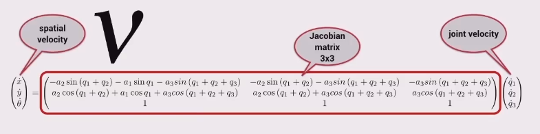
This can be written as \(v = \mathbf{J}(q)\dot{q}\)
\(v\) is the tip velocity
\(\mathbf{J}(q)\) is the Jacobian matrix
The Jacobian is the matrix equivalent of the derivative.
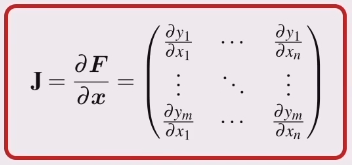
Here the Jacobian is a function of the joint angles and the kinematic parameters of the robot.
Greek letter nu, \(nu\)
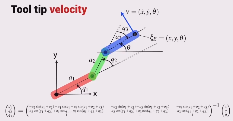
Given the end-effector velocity, what are the joint velocities?
\(\dot{q} = \mathbf{J}(q)^{-1}v\)
The Jacobian can only be inverted if it is
square: the robot’s task and configuration spaces are equal, and
non-singular: the robot’s joint coordinates avoid certain “singular” configurations.
A singular Jacobian matrix indicates that the end-effector motion is unable to move in or rotate about a particular Cartesian direction. (loss of a DOF)
A pose may be nearly singular, making movement in some directions difficult.
Can be determined by the Jacobian determinant or the Jacobian condition number.
A small determinant corresponds to a large condition number, that is, the matrix is nearly singular.
The velocity ellipse describes the ease in which the robot arm may move in either direction.
A narrow ellipse means the robot is close to a singularity.
It can be described by the equation \[\nu^T (\mathbf{J}(\mathbf{q})\mathbf{J}^T(\mathbf{q}))^{-1} \nu = 1\] Where \[\nu=(\dot{x},\dot{y})\] and \[\mathbf{\dot{q}}=(\dot{q_1},\dot{q_2})\] \[\mathbf{\dot{q}}=\mathbf{J}(\mathbf{q})^{-1}\nu\]
Moving faster in the y direction than x.
Resolved-rate motion control is a technique to move the end-effector at a specified velocity without having to compute inverse kinematics.
Choose the Cartesian velocity \(\nu\)
Find the joint velocities using the inverse Jacobian
Move the joints at that speed
At the next time step, update the Jacobian as it is a function of the joint angles, which have now changed
Goto step 2
This technique may or may not be less computationally expensive than computing the inverse kinematics at every step.
Remember a 3-joint planar arm is able to control its orientation independently of its position.
Find the forward kinematics transform matrix, then
Therefore
Also note
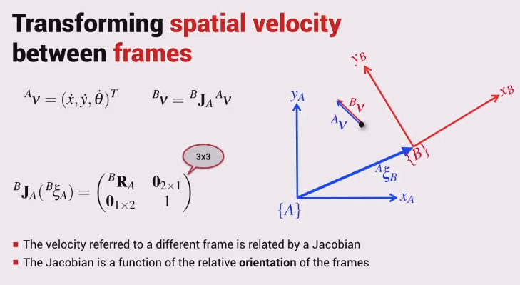
The velocity of a point relative to coordinate frame A is related to its velocity relative to frame B by a Jacobian which is a function of the rotation from frame B to frame A.
The spatial velocity \(\nu\), also called twist, is a vector of six parameters that describes the instantaneous velocity in 3D.
\[\mathbf{\nu}=(\nu_x,\nu_y,\nu_z,\omega_x,\omega_y,\omega_z)\]
Three of these elements describe the velocity of a point moving in 3D-space, and the other three describe the angular velocity of a body rotating in 3D-space.
For a 6-link robot, the previous approach to computing the Jacobian becomes unwieldy so a numerical approximation to the forward kinematic function is computed instead.
Just like when you learnt calculus
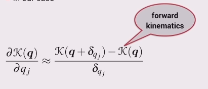
The derivative is approximated by calculating a finite difference.
What to do if you want to find the end-effectors translational velocity?
Well this can also be said to be the rate of change of translation with respect to time.
This can be found by multiplying the partial derivative of the robots position with respect to \(q_1\) and the rate of change of \(q_1\) with respect to time.
\[\frac{\partial\mathbf{t}}{\partial q_1} \frac{dq_1}{dt} = \frac{d\mathbf{t}}{dt}\]
The end-effectors translational velocity, \(\frac{d\mathbf{t}}{dt}\), can be expressed as \(\begin{pmatrix} \dot{x} \\ \dot{y} \\ \dot{z} \end{pmatrix}\) or \(\begin{pmatrix} v_x \\ v_y \\ v_z \end{pmatrix}\).
Should end with an expression like
\[\begin{pmatrix} v_x \\ v_y \\ v_z \end{pmatrix} \approx \begin{pmatrix} ? \\ ? \\ ? \end{pmatrix} \dot{q_1}\]
The same can be done for the rotational part with some differences.
Using \(\frac{\partial\mathbf{R}}{\partial q_1}\) from step 4,
\[\frac{\partial\mathbf{R}}{\partial q_1} \frac{dq_1}{dt} = \frac{d\mathbf{R}}{dt}\]
Note that \(\mathbf{\dot{R}}=\mathbf{S}(\omega)\mathbf{R}\), where \(\mathbf{S}(\omega)\) is the skew symmetric matrix.
\[\mathbf{S}^T=-\mathbf{S}\] \[\mathbf{S}^T+\mathbf{S}=0\]
Always singular \[det S = 0\]
Any matrix is the sum of symmetric and a skew symmetric matrix
In 3 dimensions 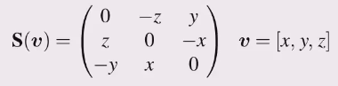
An alternative way to express the vector cross product \(\mathbf{a} \times \mathbf{b}=\mathbf{S}(\mathbf{a})\mathbf{b}\)
Continuing on from the translational section above, we have to rearrange the expression
\[\frac{\partial\mathbf{R}}{\partial q_1} \frac{dq_1}{dt} = \frac{d\mathbf{R}}{dt}\]
to get \(\mathbf{S}(\omega)\).
Take the inverse of \(\mathbf{R}\) (which is the same as the transpose for a rotation matrix) to get
\[\mathbf{S}(\omega) = \frac{\partial\mathbf{R}}{\partial q_1} \mathbf{R}^T \dot{q_1}\]
then compute numerically.
Then using our knowledge of skew symmetric matrix properties, can find \(\omega_x\), \(\omega_y\) and \(\omega_z\), then rewrite it in matrix form as
\[\begin{pmatrix} \omega_x \\ \omega_y \\ \omega_z \end{pmatrix} \approx \begin{pmatrix} ? \\ ? \\ ? \end{pmatrix} \dot{q_1}\]
Simply stack the translation and rotation vectors on top of each other to get the relationship between the spatial velocity and the velocity of the robots first joint angle.
\[\begin{pmatrix} v_x \\ v_y \\ v_z \\ \omega_x \\ \omega_y \\ \omega_z \end{pmatrix} \approx \begin{pmatrix} ? \\ ? \\ ? \\ ? \\ ? \\ ? \end{pmatrix} \dot{q_1}\]
\[\begin{pmatrix} v_x \\ v_y \\ v_z \\ \omega_x \\ \omega_y \\ \omega_z \end{pmatrix} \approx \text{[6x6 matrix] } \begin {pmatrix} \dot{q_1}\\\dot{q_2}\\\dot{q_3}\\\dot{q_4}\\\dot{q_5}\\\dot{q_6} \end{pmatrix}\]
The 6x6 matrix is a Jacobian matrix, referred to as the manipulator Jacobian matrix.
Can alternatively express this as \(\nu = \mathbf{J}(\mathbf{q})\mathbf{\dot{q}}\).
Each column of the Jacobian matrix is the contribution by the robots joint \(i\) to the end-effectors spatial velocity. Add them together to get the total end-effector spatial velocity.
The Jacobian matrix can be inverted so long it is
(see here)
The inverse Jacobian allows us to determine the joint velocity given the end-effector velocity.
This technique is same as for the 2D situation except the joint velocity is computed as \(\mathbf{\dot{q}}=\mathbf{J}(\mathbf{q}_k)^{-1}\nu\)
Similar to the 2D case.
The Jacobian can be used as a diagnostic tool to find out how well the robot’s configuration is suited to the task.
If two columns of the Jacobian are the same, say columns 4 and 6, then the Jacobian is singular (the motion of joints 4 and 6 results in the same motion).
If the ellipsoid is a sphere
Manipulability is defined as
\[ m=\frac{\min R}{\max R}, 0 \leq m \leq 1\]
where
(The-2D-case)
![]()
The spatial velocity of a body relative to coordinate frame A is related to its velocity relative to frame B by a Jacobian which is a function of the rotation from frame B to frame A.
We can use the spatial velocity transform to compute an alternative manipulator Jacobian matrix that maps joint velocity to end-effector spatial velocity in the end-effector coordinate frame.
The analytic Jacobian relates change in roll-pitch-yaw angles to angular velocity.
We can re-express the spatial velocity using the analytic Jacobian \(\mathbf{J}_a\).
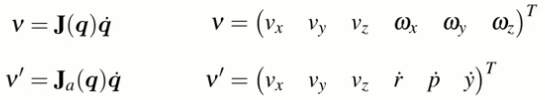
where \(\mathbf{J}_a\) is
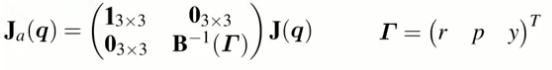
and
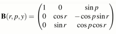
Jacobian: 6 rows, N columns (number of joints)